CoNIFER Tutorial:
This is a general tutorial for using CoNIFER. If you are interested in just giving CoNIFER a spin with the included test
data, read the Quick Start Guide.
General command structure and getting help
CoNIFER is a command-line python program (conifer.py). There are several sub-commands, each with a set of command line options. In general, the CoNIFER pipeline consists of the following steps:
1. Calculate RPKM values for all samples
2. Analyze all RPKM values for all samples and create SVD-ZRPKM values. This steps create a single unified conifer data file which contains all data, probes and samples for downstream analysis.
3. View, make calls or export SVD-ZRPKM values for segmentation using other/existing algorithms
Not all steps are required. For example, Step 1 is only needed if you wish to transform a set of .bam alignment files into RPKM files. If you have RPKM files created from another source, you can omit step one (bamToRPKM.py).
Help and available command line options for any of these steps can be listed using the --help or -h options, e.g.:
1. Calculate RPKM values for all samples
python conifer.py rpkm [...]
2. Analyze all RPKM values for all samples and create SVD-ZRPKM values. This steps create a single unified conifer data file which contains all data, probes and samples for downstream analysis.
python conifer.py analyze [...]
3. View, make calls or export SVD-ZRPKM values for segmentation using other/existing algorithms
	python conifer.py export [...]
	python conifer.py call [...]
	python conifer.py plot [...]
	python conifer.py plotcalls [...]
Not all steps are required. For example, Step 1 is only needed if you wish to transform a set of .bam alignment files into RPKM files. If you have RPKM files created from another source, you can omit step one (bamToRPKM.py).
Help and available command line options for any of these steps can be listed using the --help or -h options, e.g.:
python conifer.py analyze --help
0. Requirements and Setup
CoNIFER requires Python v2.7 (Python 3 is not yet supported) In addition, the NumPy and PyTables packages must be installed for CoNIFER to work. If you wish to generate RPKM files from BAM alignments, pysam is required as well.
Finally, for plotting images, CoNIFER uses matplotlib.
1. Create probe/target definition file
This file defines the chr:start-stop coordinates for the probes/targets in the exome capture. We suggest basing this off the published target files from the vendor, but a custom file may be necessary for some designs.
You can download the standard probe file used in Krumm et al. here. Otherwise, the probes.txt file should be a tab-delimited file with the following header and columns:
chr	start	stop	name
1	69090	70008	OR4F5
1	565876	566576
1	801642	802733
1	861321	861393	SAMD11
1	865534	865716	SAMD11
1	866418	866469	SAMD11
1	871151	871276	SAMD11
1	874419	874509	SAMD11
1	874654	874840	SAMD11
Note: You do not have to include a "genes" column, but without it, it will not be possible to plot genes and gene names.
2. Create RPKM files
CoNIFER can calculate RPKM from aligned and indexed BAM files using the python pysam package.
  python conifer.py rpkm \
	--probes probes.txt \
	--input sample.bam \
	--output RPKM/sample.rpkm.txt
All of the RPKM files you wish to analyze in a CoNIFER experiment should be placed in a single directory, without any other files.
3. Main CoNIFER analysis:
In this step, the RPKM files are loaded into memory, poorly responding probes are masked, and the Z- and SVD- transformations are applied. The final SVD-ZRPKM values for each exon are stored in a unified HDF5 file.
Although this analysis is single-step process, users will generally need to repeat this step at least once in order to choose the correct number of SVD components to remove, as well as eliminate any poorly performing samples (see Quality Control of Exomes, below).
To run the analysis, use the command "analyze":
Each of the options is explained below:
--probes: location of probe file
--rpkm_dir: the directory containing the previously generated RPKM files.
--output: the location/filename of the CoNIFER output analysis file.
--svd: the number of SVD components to remove (zero). See below for more on this subject.
--write_svals: when set, CoNIFER will output the singular values from the SVD analysis for plotting in a scree plot.
--plot_scree: when set, CoNIFER will use matplotlib (required for this option) to create a scree plot of the singular values in the data.
--write_sd: when set, CoNIFER will calculate the overall standard deviation for each sample and output them in the indicated text file.
Plotting singular values (NEW in CoNIFER 0.2.1) After running the analysis withthe --plot_scree or --write_svals option, examine either the scree plot or the SVD values in the singular_values.txt file themselves (you can easily recreate the scree plot using any popular visualization tool, such as Excel) Below is the output of the --plot_scree command when analyzing the sample dataset of 26 rpkm files:
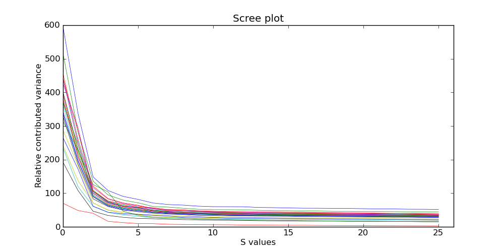
We recommend selecting the number of SVD components removed (--svd) based on the inflection point or the plateau of the scree plot. For the dataset above, --svd 2 up to --svd 5 would be approriate. In general, values of 3-20 should be considered, depending on the size and the amount of systematic variance found within the dataset. See the manuscript for more details.
Quality Control of Exomes: Poorly performing exomes can be found by examining the standard deviation values in the sd_values.txt file. These values are the standard deviations of all SVD-ZRPKM values for each individual. Plotting the ordered values can quickly show which samples are outliers. NOTE: For optimal performance, we recommend pruning samples with extremely high standard deviation values from the analysis, and re-running the analyze step with only QC-passing samples.
  python conifer.py analyze \
  	--probes probes.txt \
  	--rpkm_dir ./RPKM/ \
  	--output analysis.hdf5 \
  	--svd 6 \
  	--write_svals singular_values.txt \
  	--plot_scree screeplot.png \
  	--write_sd sd_values.txt
Each of the options is explained below:
--probes: location of probe file
--rpkm_dir: the directory containing the previously generated RPKM files.
--output: the location/filename of the CoNIFER output analysis file.
--svd: the number of SVD components to remove (zero). See below for more on this subject.
--write_svals: when set, CoNIFER will output the singular values from the SVD analysis for plotting in a scree plot.
--plot_scree: when set, CoNIFER will use matplotlib (required for this option) to create a scree plot of the singular values in the data.
--write_sd: when set, CoNIFER will calculate the overall standard deviation for each sample and output them in the indicated text file.
Plotting singular values (NEW in CoNIFER 0.2.1) After running the analysis withthe --plot_scree or --write_svals option, examine either the scree plot or the SVD values in the singular_values.txt file themselves (you can easily recreate the scree plot using any popular visualization tool, such as Excel) Below is the output of the --plot_scree command when analyzing the sample dataset of 26 rpkm files:
We recommend selecting the number of SVD components removed (--svd) based on the inflection point or the plateau of the scree plot. For the dataset above, --svd 2 up to --svd 5 would be approriate. In general, values of 3-20 should be considered, depending on the size and the amount of systematic variance found within the dataset. See the manuscript for more details.
Quality Control of Exomes: Poorly performing exomes can be found by examining the standard deviation values in the sd_values.txt file. These values are the standard deviations of all SVD-ZRPKM values for each individual. Plotting the ordered values can quickly show which samples are outliers. NOTE: For optimal performance, we recommend pruning samples with extremely high standard deviation values from the analysis, and re-running the analyze step with only QC-passing samples.
Making calls:
The current version of CoNIFER implements a rudimentary CNV detection algorithm based on SVD-ZRPKM thresholds (as implemented for the description of ConIFER in Krumm et al., 2012). However, the SVD-ZRPKM values for each sample are well-behaved array-like datapoints, which can be integrated into various segmentation algorithms (e.g., CGHCall, HMMs, etc).
To make calls using the CoNIFER threshold algorithm:
To make calls using the CoNIFER threshold algorithm:
  python conifer.py call \
  	--input analysis.hdf5 \
  	--output calls.txt
Exporting data for segmentation and viewing:
To export ALL samples:
  python conifer.py export \
  	--input analysis.hdf5 \
  	--output ./export_svdzrpkm/
or a single sample:
  python conifer.py export \
  	--input analysis.hdf5 \
  	--sample SampleID \
  	--output ./export_svdzrpkm/sample.svdzrpkm.bed
Printing and viewing CoNIFER data:
CoNIFER comes with simple routines that make visualization of the SVD-ZRPKM data simple. The plotting routines are based on matplotlib and PyPlot, which are required for these features.
To plot an arbitrary segment of the exome :

Legend/Explanation:
X-axis: Exons/probes from the probes.txt file
Y-axis: SVD-ZRPKM values for each exon.
Red bars and line: SVD-ZRPKM values for each exon from the sample with the call (or highlighted sample). The smooth continuous line is simply a gaussian-smoothed representation of the SVD-ZRPKM values at each exon.
Thin black in background: All other samples in the analysis (for comparison and simultaneous visualization purposes)
Purple bars: Genes from the probes.txt file
Black bar: If using the "plotcalls" command, this bar will indicate extent of call above threshold (--threshold) value.
Multiple samples can be highlighted at once using the following notation:
Finally, if a calls.txt file is available, all the regions can be plotted in one pass using the plotcalls command:
  python conifer.py plot \
  	--input analysis.hdf5 \
  	--region chr#:start-stop \
  	--output image.png \
  	--sample sampleID
The result is shown below:
Legend/Explanation:
X-axis: Exons/probes from the probes.txt file
Y-axis: SVD-ZRPKM values for each exon.
Red bars and line: SVD-ZRPKM values for each exon from the sample with the call (or highlighted sample). The smooth continuous line is simply a gaussian-smoothed representation of the SVD-ZRPKM values at each exon.
Thin black in background: All other samples in the analysis (for comparison and simultaneous visualization purposes)
Purple bars: Genes from the probes.txt file
Black bar: If using the "plotcalls" command, this bar will indicate extent of call above threshold (--threshold) value.
Multiple samples can be highlighted at once using the following notation:
  python conifer.py plot \
  --input analysis.hdf5 \
  --region chr#:start-stop \
  --output image.png \
  --sample r:sampleID1 b:sampleID2 g:sampleID3
The first sample is highlighted in red, and the second and third will be plotted in blue and green, respectively.
Finally, if a calls.txt file is available, all the regions can be plotted in one pass using the plotcalls command:
  python conifer.py plotcalls \
  	--input analysis.hdf5
  	--calls calls.txt
  	--outputdir ./call_imgs/